Excel - Dynamic Drop Down Lists with Full Validation
15 Mar 2009I was recently asked to look at a problem a colleague was having with an
Excel spreadsheet where they wanted to use a drop down list in the cells
of one column and then a drop down list in the next column that was
dependent upon the selection in the previous column. This is something
I’d come across before and a little browsing of the help file refreshed
my memory and I gave them a solution based upon data validation and the
use of the INDIRECT function.
Here’s an example:
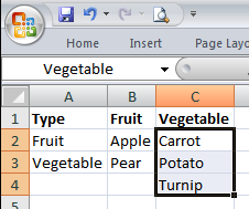 First of all I’ve created a worksheet with some lists
that will be used to drive my data validation lists. The three lists are
“Type”, “Fruit” and “Vegetable”. I’ve not exactly been clever with this
but I have applied a couple of things to make this easier.
First of all I’ve created a worksheet with some lists
that will be used to drive my data validation lists. The three lists are
“Type”, “Fruit” and “Vegetable”. I’ve not exactly been clever with this
but I have applied a couple of things to make this easier.
The first is that I have named the cells in each column relating to the list. Providing a name makes it easy to reference particularly when I’m holding the lists on a different worksheet to where I’m going to be doing the data validation.
The second is the names I have chosen. If we take type as the ‘primary’ list from which the other two ‘secondary’ lists are being selected I’ve named the secondary lists precisely as the items are displayed in the primary list. I’ve put the name of each list selection in the top cell of each column to make it even more explicit, but this means I don’t have to do any cross referencing or special look-ups later.
Next on my main worksheet I set up a couple of data entry columns. The first is for food and the second for a more detailed selection of the type of food. To set the first column to use an appropriately validated drop down list I select Data Validation from the Data menu (in Excel 2007 at least) and then select to use a list to validate and point to the named range “Type” as the source of the list using the INDIRECT function.
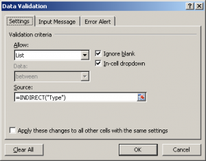
My selection is limited to the values in the named range of “Type”, and should I try to enter something else into that cell I get an error message - just the default one in this case though it can be customised on another data validation tab.
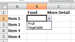
I now set-up the data validation for the
“More detail” column in the same way as the “Food” column, but this time
instead of using =INDIRECT("Type") as my list data source for data
validation I instead use =INDIRECT(B2) for cell C2, and then
replicate this down to the cells below (C3 references B3, etc.)
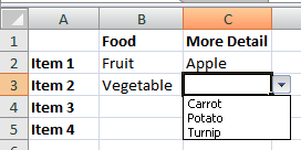
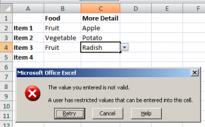
Here the drop down lists will now vary in accordance with the food that has been chosen in the previous column. Errors for the lists also seem to be intact as if we select the “Food” entry as being ‘Fruit’ and then try to type in a choice that is not in the list (in this case ‘Radish’ which isn’t in any of the lists, but it could actually be anything other than ‘Apple’ or ‘Pear’ in this example) we get a familiar looking error message.
At this point it looks like we have a simple and effective solution. But this is where I began to be a bit more thorough in my testing than I think many others have been. Specifically what happens when we don’t have a food entry?
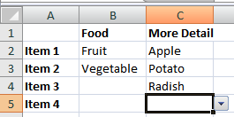
Clicking on the drop down doesn’t display any list entries for selection - because it is just an empty list. Typing an entry in however is accepted as there is nothing being validated against - as shown in cell C4. This is a bit of a problem … but you’ve probably figured out buy now that I have a solution.
My original solution attempt was to change the source by checking if the food type had been entered and if it had then returning a blank list, otherwise the appropriate secondary list.
Taking cell C4 as my working example…
=INDIRECT(B4)
… was changed to …
=IF(B4="","",INDIRECT(B4))
Unfortunately this yielded the same result in terms of the behaviour
observed. I also tried replacing the conditional parameter of B4=""
to ISBLANK(B4), but again this made no difference.
Next I tried replacing the list to use when B4 is blank with another
list using the following data validation list source statement
=IF(B4="","BLANKLIST",INDIRECT(B4)). The list BLANKLIST did not
exist but again the same result. Again I tried using ISBLANK(B4),
and again no difference.
I created the BLANKLIST named range with one entry of “N/A”, but the
only difference this made was that when the food entry was blank the
more detail list now had one option of “N/A”, but still anything could
be types into the cell without a warning message.
As well as having the IF as the outer most function I also tried the
various combinations with INDIRECT as the outermost function…
=IF(B4="","",INDIRECT(B4))
… became …
=INDIRECT(IF(B4="","",B4))
… and so on for each of the options described above (which was quite a few!) but still nothing worked. Overall exceedingly odd behaviour when it is compared to what is happening in the cells above if something is entered that is not in the data validation list. This may be a bit of a bug in Excel’s data validation processing.
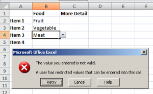
In the end I split out my conditional processing from my data validation processing. This could be put onto a separate hidden worksheet or into a hidden column. For this example I’ve just placed it next to the more detail column.
Cell D4 contains the following function:
=IF(B4="","",B4)
Cell C4 then contains the following for its data validation list source:
=INDIRECT(D4)
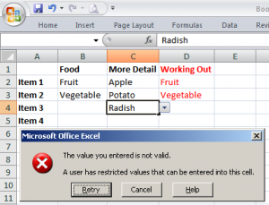 The data validation finally works as expected
enforcing the more detail entry to be from the appropriate secondary
list unless the food entry is blank in which case no entry is allowed.
Not the prettiest solution, but one which allows your dynamic drop down
lists to maintain the enforcement of data validation where the primary
data selection has not been made.
The data validation finally works as expected
enforcing the more detail entry to be from the appropriate secondary
list unless the food entry is blank in which case no entry is allowed.
Not the prettiest solution, but one which allows your dynamic drop down
lists to maintain the enforcement of data validation where the primary
data selection has not been made.
If you want a copy, you can also download an example spreadsheet.