Auto Incrementing in Excel
29 Jun 2013In this post I’m going to share a tip about auto incrementing numbers in Excel. I’ve frequently found myself creating incremental number lists (e.g. 1, 2, 3, 4, 5, …, etc.) and whilst Excel is quite helpful at providing ways to create such lists I find its methods are often a bit limited for my needs - so I came up with another way that I think you might find more resilient.
Typical Methods
So many Excel users are probably familiar with a few common ways to create incremental lists. In all of the methods I’ll describe below I’ll describe them as vertical lists, but they could just as easily be horizontal lists.
Auto-fill
- Enter the value 1 into a cell.
- Enter the value 2 into the cell beneath it.
- Select the two cells.
- Left click on the small square in the bottom right corner of the second cell and drag it down to the cell you wish to be the end of the series.
Excel will fill each cell with the incremental numeric value.
Basic Formula Fill
- Enter the value 1 into a cell (e.g. into C2).
- Enter a formula to add 1 to the value in the cell above (e.g. =C2+1).
- Select from the second cell down to the last cell in the series and press CTRL+D to fill down.
Excel will fill each cell with a formula to take the cell above and add one to it.
The Issue
Let me be clear at this point. These methods work absolutely fine. The issues occur when you choose to insert, duplicate and/or remove rows.
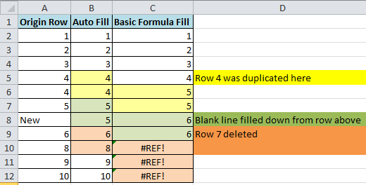
- Duplicating Rows
- Auto fill: produces identical number to the row from which it was duplicated.
- Basic Formula Fill: produces identical number to the row from which it was duplicated.
- Inserting Rows (and fill down from row above)
- Auto fill: produces identical number to the row above.
- Basic Formula Fill: produces the number of the row above incremented by 1.
- Deleting Rows
- Auto fill: subsequent rows will keep the same number as they had previously.
- Basic Formula Fill: subsequent rows will return an error.
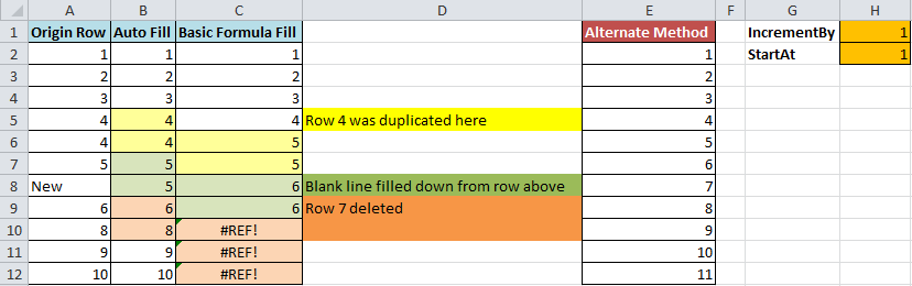
Alternate Method
With the methods described above you quickly start getting confusing results. The solution in each case is to simply regenerate the series by repeating the process to populate it. I find this tedious and in many cases it messes around with formatting (particularly conditional formatting) that I have in place. So my solution is to use a more complex but flexible formula and here’s how it breaks down.
The first step is one that is based on an assumption … but one that works for me and the way I tend to structure my spreadsheets. The assumption is that when a list is to increment, the cell above will be a number. So if there is text in the cell above or there is no cell above (i.e. it is in row 1) then it is the first cell in the list. For this first pass through we’ll assume our list starts at 1 and so our pseudo-Excel formula is as follows.
=if(isnumber({cell above},{cell above}+1,1)
Note that we have two entries for {cell above}. Here’s where we apply the resilience - rather than specifying a specific cell we need to make the reference a relative one.
The Excel function that allows us to fetch a value for a relative cell
is INDIRECT. This function takes a cell reference so we still need to
provide the actual cell reference. The ADDRESS function allows us to do
just that, but it requires a row and column.
So we can redefine the {cell above} place holder as follows.
{cell above} = INDIRECT(ADDRESS({row above},{same column}))
This means that the overall pseudo-Excel formula becomes…
=if(isnumber(INDIRECT(ADDRESS({row above},{same column})),INDIRECT(ADDRESS({row above},{same column}))+1,1)
Excel fortunately provides the ROW and the COLUMN function. These
functions return the current row and current column of the cell
respectively.
We can use a simple subtraction to reference a previous row.
{row above} = ROW()-1
The {cell above} place holder would thus become.
{cell above} = INDIRECT(ADDRESS(ROW()-1,COLUMN()))
So the resulting formula becomes…
=if(isnumber(INDIRECT(ADDRESS(ROW()-1,COLUMN())),INDIRECT(ADDRESS(ROW()-1,COLUMN()))+1,1)
You can also extend the formula to be a little more flexible by replacing the last two “1”s with references to named cells. To name a cell simply over-type the cell ID (e.g. A1) with the name you wish to use.
So we change the formula like so.
=IF(ISNUMBER(INDIRECT(ADDRESS(ROW()-1,COLUMN()))),INDIRECT(ADDRESS(ROW()-1,COLUMN()))+IncrementBy,StartAt)
- IncrementBy - the number by which to increase the number by with each row.
- StartAt - the value of the first number in the list.
Hopefully you can follow the logic behind this, but if not then you can probably get away with just copying and pasting in the formula.
When you apply the duplicate, inserted (and filled down) and deletion of rows, the result is that the new method retains the incremental structure.
You can also download an example spreadsheet (XLSX) with the comparison of the techniques including the extended formula.